Re-linearising A Piezo Curve

This article is definitely advanced.  It will only really make sense to people already using Piezography, although technically-minded potential users may find it helpful to know that re-linearisation can now be done.  The fact that it wasn’t readily possible, before mid-2015, was a turn-off for some people considering Piezography.  Note that in order to re-linearise a curve you will need a measurement device.

The Problem

If you create a curve for QuadToneRIP (QTR) using the curve creation tools that come with QTR, then you create a QTR Ink Descriptor File (.qidf on Windows but a .txt file on Mac OS X) that specifies the basic parameters of the curve.  QTR then “compiles” this into a .quad file, which lists the amounts of each ink channel that are used in printing.  If you need to adjust the curve, including to re-linearise it, then you edit the .qidf/.txt file and QTR will recompile the .quad file.  There are a number of tutorials available about how to do all this.

The catch with Piezography is that its curves are not produced this way.  There are no .qidf/.txt files to edit.  You only have the .quad file.  So if you want to tweak the curve, or if you need to re-linearise it, until recently you couldn’t.  Well, not easily.  There were some complicated approaches developed using spreadsheets, but these were not for the faint-hearted or non-technically minded.

So if you wanted a Piezography curve for a paper not currently supported, or you measured an existing curve on your printer and found it to be excessively non-linear, your only option was to pay InkJetMall $US99 per curve.  It also meant posting printed sheets to the US and waiting …..  And this wasn’t even an option in some cases (Piezography 2 on the R1900 and R2000).

The Solution

In mid-2015, the creator of QTR, Roy Harrington, created a small “droplet” application that will “re-linearise” an existing .quad file.  As Roy says in that thread, the droplet is only doing what you’d do in QTR itself to re-linearise a curve, if you had a .qidf/.txt file to work with.  Thus the droplet seems to formalise a cumbersome spreadsheet technique that I had developed.  The droplet is so much easier, and more accurate as well.

Unlike the other droplet applications that come with QTR, which you can locate on the desktop for easy dragging and dropping, this one must be installed in the the QTR binary folder.  On Windows this is “C:\Program Files (x86)\QuadToneRIP\bin\QTR-Linearize-Quad.exe” and on Mac OS X it is “/Applications/QuadtoneRIP”.  Since QTR 2.7.6.0,  the re-linearisation droplet is installed in the correct place with QTR.

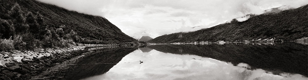
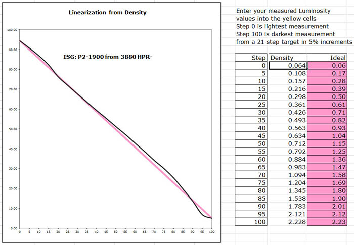
Here is an example of a P2 curve for Canson Rag Photographique that, while not too bad, clearly needs re-linearisation:

To use it:

1. In Windows, I find that the easiest way to run the droplet is to create a shortcut to it on the desktop.  On Mac OS X, I’m reliably advised that you can launch it as needed from the QTR folder.
2. Use QTR to print out a set of standard patches, like the 21×4 set, using the curve you want to linearise on the paper in question.
3. Measure the 21×4 and save the measurement data in a working folder.  I find it convenient to save a copy of the .quad file that you’re re-linearising in the same folder, for the next step.
4. Select both the measurement data file and the .quad file copy and simultaneously drag them both onto the droplet shortcut.
5. You’ll get two files created in the working folder:  an “out” text file with the linearisation outcome, and an xxxx-lin.quad file, which is the re-linearised curve.  (The linearisation outcome data in the “out” text file only shows the status of the curve before re-linearisation, not after, so it doesn’t provide any indication how successful the re-linearisation was.  For that you must do steps 6-8.)
6. You could just print with this curve, but before you do, I’d strongly suggest you check that it’s linear, as some curves can cause the droplet to fail or produce decidedly odd results (see below).
7. So repeat steps 2 and 3 using the re-linearised curve, and the drop the second stage measurement data onto either QTR-Linearize-Data.exe, QTR-Create-ICC.exe or QTR-Create-ICC-RGB.exe (without the .exe at the end for Mac OS X).
8. Insert the output data from the second stage “out” file into the linearisation checker spreadsheet to check that you have a linear curve (an updated version of the spreadsheet is now found in the Piezography Community Edition, but the original version you see displayed in graphs in these pages is still available here).
9. If you do, then copy or move the re-linearised.quad file into the folder of quad files for your printer.  On Mac OS X, there’s a re-installation dance that you’ll have to perform.

[Note:  this discussion implicitly assumes that you measurement device is an i1Photo.  If you have a ColorMunki, then read this article in conjunction with the how-to for using a ColorMunki.]

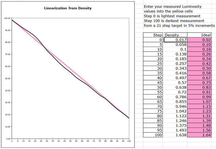
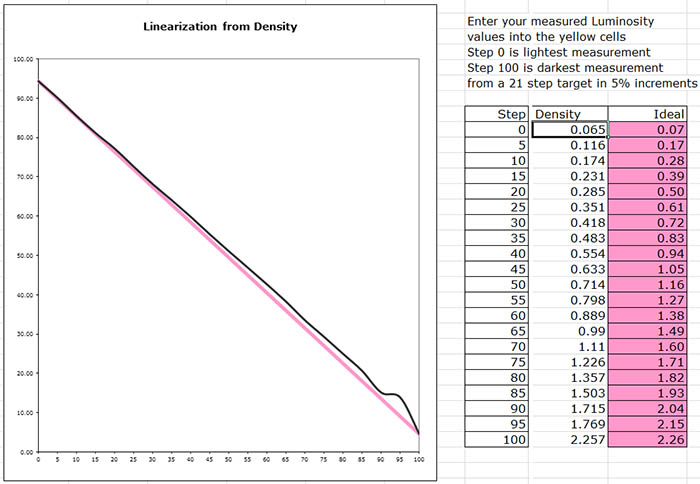
Here is a the re-linearisation of the P2 curve for that Canson Rag Photographique curve:

Does It Work?

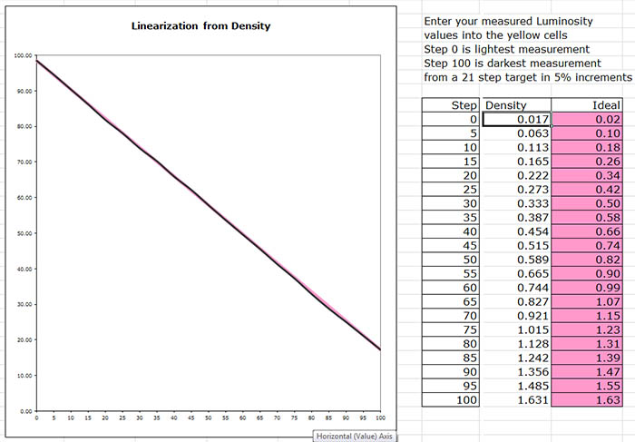
At one level, the answer to this question is yes.  If you look at that plot just above, the re-linearised CRP curve is very linear.  At another level, the question might be rephrased as: how different is the re-linearised curve from one that InkJetMall might produce using their custom curve creation service?  That I don’t know.  I’ve never done one then the other.  If you look at the underlying structure of re-linearised curves, and compare them to IJM-produced curves, the IJM ones do seem to be a bit smoother than the re-linearised ones, although not always.  The real test is in the prints, and I think that prints made using re-linearised curves look just fine.  I can’t see any artefacts.

Moreover, you can use the droplet to create curves for unsupported papers.  For example, there’s no Piezography 2 curve for Innova Smooth Cotton High White (ISCHW).  I took the curve for Hahnemuhle Photo Rag (HPR) and successfully used it as the starting point for the above re-linearisation process for ISCHW.  If you have trouble finding a suitable starting point, or if you simply want the best result, you can print the 21×4 using a range of candidate curves and select the best.  The closer the starting point, the less work the droplet has to do and the smoother the underlying structure of the re-linearised curve is likely to be.  But normally all you need is another reasonably similar curve to use as a starting point.  So the droplet really opens up a range of opportunities to be self-sufficient.

Problems

The re-linearisation droplet has its limitations.  If the wiggles in your non-linear curve are excessive, then the mathematics behind the re-linearisation will fail, or in some cases will make matters worse.  Sometimes you’re just plain out of luck.

Here’s an example of a problematic curve for Ilford Smooth Pearl with too much of a dip in the shadows:

And here is what the re-linearisation droplet resulted in:

which is definitely worse.  I had to straighten out this curve in a two-stage process, but that’s another story.

Last: To Convert or Not Convert?

Next: Relinearising Piezography Curves with a ColorMunki